From the series Introduction to Analysis for Designers...
The most common analyses designers perform are strength stiffness analysis, thermal analysis and eigenvalue analysis. The boundary conditions for each one of these analyses are different and they will depend on the setting of loads and constraints. In this chapter, we will examine the influence of boundary conditions, which are at the core of the designer’s choices, on the analysis results.
First, let us define what boundary conditions are. Setting boundary conditions on a designed object is simply determining the environment around it, and the external factors that are expected to act on it, to be able to analyze its behavior. For example, a boundary condition can define, among many other things, how a structure is to be fastened with a bolt, fixed with a weld or supported with an insert, or where to apply a force, or whether to push or pull an object. Even if the shape and physical properties of an object remained the same throughout different analyses, the actual stress and deformation on such object will vary greatly depending on the boundary conditions.
In general, in structural analysis, boundary conditions are of two types:
The load condition is relatively easy to understand, even for beginners; the magnitude and direction of a set load, and the position where the load acts, are concepts easy to grasp. However, the setting of constraints often brings confusion. Let’s then see what types of constraints there are.
Typical examples of constraints are:
Designers familiar with CAE software may think it is easy to set the boundary conditions for the supports mentioned above. However, if not approached carefully, they might fall into unforeseen troubles in the analysis. It is no exaggeration to say that the accuracy of analysis results depends greatly on how the constraints are determined.
The model of a hook-shaped joint structure, introduced in the previous chapter to illustrate the meshing process, will be used here again as an example. Usually, a joint structure of this kind is bolted to a wall and used by applying a load to the top surface of the hook. In this model, a hole for a bolt already exists, and we to set a boundary condition on it, as shown in Fig. 1.
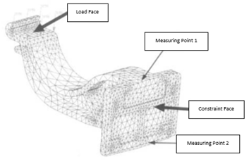
Figure 1: Constraints on a Joint Structure Analysis Model: The right-side plane was fixed, and the load was applied from the left end downwards.
The first consideration needed is the stiffness of the wall that holds the structure. Although one might focus only on the object of analysis and overlook this, setting boundary conditions goes beyond understanding the object and where its constraints and loads are. Under the prescribed conditions, the stress generated in this structure will change completely according to the rigidity of the wall it is attached to.
In order to accurately analyze the strength and stiffness of the designed object, the stiffness of the objects that constrain it must also be interpreted. For example, consider the extreme case of a soft wall and a rigid structure. As you can imagine, if the wall is soft, the deformation load from the stiffness balance between the structure and the wall will be biased towards either one of the two, depending on the load acting on the joint. On the other hand, in the case of a steel wall, only the joint structure tends to bear the load.
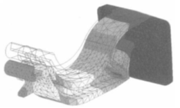
Figure 2: Example of Analysis Results for a Joint Structure
Let’s now observe the effect of boundary conditions on the results. For the sake of simplicity, we assume the wall is rigid and two possible settings of constraints. If the first setting is applied, the entire contact surface of the structure would be fixed and the stiffness of the bolts holding it is assumed infinite; we will name this the “whole fixed model” constraint setting. The second one assumes only the bolt hole is fixed; we will refer to it as the “bolt model” setting. In practice, the joint structure is fixed to the wall with bolts. However, if the bolt tightening torque is considered sufficient, and the bolt is judged to be strong enough, the “whole fixed model” is often used to simplify the analysis.
For each setting of constraints, we will now compare results from two types of joint structures with different stiffness: one made of iron, the other of aluminum. You can see a representative example of the analysis results in Fig. 2.
Let us first pay attention to the results of the analysis of the “bolt model” setting: the displacement of the joint structure outwards from the wall at Measuring Point 1, and the displacement of the joint structure inwards into the wall at Measuring Point 2. In both the iron model and the aluminum model, the load conditions are the same. As shown in Fig. 3, although the direction of deformation is the same for both materials at each point, the magnitude of such deformation varies greatly depending of the stiffness of the structure’s material. Since the wall is rigid, the displacement at Measuring Point 2 should be zero, but it appears to be slightly inside the wall. This is due to the fact that the restraint plane, the contact surface between the joint structure and the wall, is only partially fixed and its behavior is calculated with the absence of a wall. Therefore, the displacement at this point, an at Measuring Point 1, will be larger as the stiffness of the structure analyzed becomes smaller.
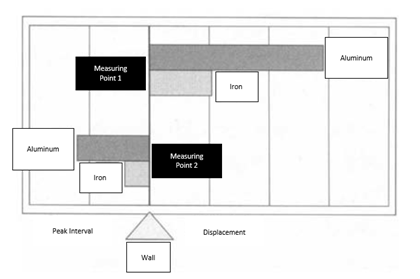
Figure 3: Displacement-from-the-wall Comparison. The magnitude of deformation depends on the rigidity of the joint structure. Since the wall is assumed to be a rigid body, the amount of deformation of aluminum, which has low rigidity, will be larger.
On the other hand, in the case of the “whole fixed model” setting of constraints, the contact plane between the structure and the wall is restrained to not move at all, so there won’t be a gap between Point 1 and Point 2 in their displacement, neither outwards nor inwards from the wall. However, as you can imagine, since the contact plane is completely fixed and Point 1 is a bit below the contact plane, there is now a gap between Point 1 and the wall. In other words, neither the “bolt model” nor the “whole fixed model” can produce completely accurate results.
Therefore, to obtain a more rigorous solution, it is desirable to set boundary conditions such as not allowing the structure to go into the wall, and conditions that account for the area where there could a gap between the wall and the joint structure. Once set, what is the validity of “whole fixed model” or the “bolt model” in the range used by the designer?
The number of bolts used and their rigidity and that of the wall must be taken into consideration. If the rigidity of the wall and bolts is high and the tightening torque is enough, it is acceptable to use the “whole fixed model.” On the other hand, if the number of bolts is small, it is better to assume a “bolt model” constraint setting.
The most important part here is estimating, to some extent, the tendency of the results by calculating certain boundary conditions, and to check whether the calculation results match what is expected of that set of boundary conditions. Boundary conditions should be set up in anticipation, to some extent, of the calculation results, rather than setting them blindly. Without the necessary training on the part of the user, the CAE software cannot fully satisfy the required analytical techniques when implemented on a certain design. At such time, design knowledge and experience are more important than the power or breadth of the CAE software.
Let’s now consider a situation where the wall stiffness is considerably low. In this case, assuming a load is applied, the wall and join structure deform simultaneously. However, since the deformation of the wall surface must now be considered, it is necessary to perform assembly analysis. Assembly analysis would imply that the wall surface is also modeled as an object to be analyzed, and that the modeled wall and join structure are then combined and analyzed as an assembly. This type of analysis is of a somewhat higher difficulty, but you should be able to easily perform it in most of CAE software.
It is natural that the lower the stiffness of the wall surface the less deformation the joint structure will undergo. Accurate calculation of this behavior requires careful attention to the setting of the contact conditions of the assembly, so it is wise to proceed with the help of expert advice. It is also important to know that, since the rigidity of the wall is low, there is no significant difference between the case where the wall is fixed to the whole contact surface and the case where it is fixed only to the vicinity of the bolt holes with respect to their interaction with the wall.
We have described the constraint conditions corresponding to bolted joints in a joint structure, but how should we set these conditions for welding, rivet, adhesion or other fitting options besides bolt joint? Welding and adhesion can be set as “whole fixed model”, due to their adaptability and shear strength. In the case of welding, however, the reaction force of the fixed front calculated must be checked to ensure it doesn’t exceed the welding strength post treatment; this can be done in the post-processing stage of the analysis. For rivets, the most fitting process is that of the “bold model”, and it is also necessary to confirm that the reaction force doesn’t exceed the strength of the rivet. For this cases, it is better to consult a CAE specialist for interpretation.
By understanding the above-mentioned reaction force state, it is possible to easily find out the load burden ratio of the component set, which is very important for designing the assembly. When designing a part, the designer assumes, or calculates, how much load is applied to the part of interest. If this assumption is incorrect, the actual balance of the load acting on the product, including that part, will be different. When you can see the state of the reaction force, it is always good to know how much load is applied to the part.
Next, the effect of constraints on the stress results is examined. Most designers find the value of maximum stress undergone by their inventions from the analysis results. This maximum stress is likely to occur where the boundary conditions have been set. From basic knowledge, you may even be aware that stress is likely to occur in areas where the stiffness changes drastically.
In the case of the bolt model, assuming the wall as a rigid body, the bolt hole was constrained as fully fixed. This complete fixation is equivalent to setting the object of study, the bolt, to have infinite rigidity. Therefore, in this case, a considerably large stress will be generated near the area where the boundary condition is set. This issue can often be avoided if the analysis model is created by translating the CAD data into the CAE software. That way, the constraint set on the face or edge of the model is automatically distributed to a plurality of nodes, reducing the likelihood of an unnatural local concentration of stiffness.
However, some CAE software, or certain analytical models, require users to directly assign conditions to nodes. Special attention should be paid to the fact that the constraints will then be set to only one or a few of the nodes, resulting in unexpected local stresses, and that the constraint force will be generated all in the constraint section. Due to this phenomenon, the maximum stress value found in the analysis results needs to be carefully examined to assure it is consistent with the strain or stress distribution in the whole model.
In addition, when the whole surface is completely fixed, it is also necessary to pay attention to the fact that the stiffness becomes considerably large near the constrained surface, making it difficult to deform and turning the stress larger than the its actual value. Although it is not very realistic, to simplify the explanation, let’s take as example the calculation of the deformation in a pipe with a U-shaped cross section when applying a load from the top surface. In Fig. 4 (a), the rigidity around the right-end face can be seen to be larger than that of the left-end face due to the fact that the right-end face is fully fixed. On the other hand, as shown in Fig. 4 (b), the pipe deforms uniformly because both ends are free to deform freely in the vertical direction. This exemplifies that the constraint setting can make the analysis results vary greatly.
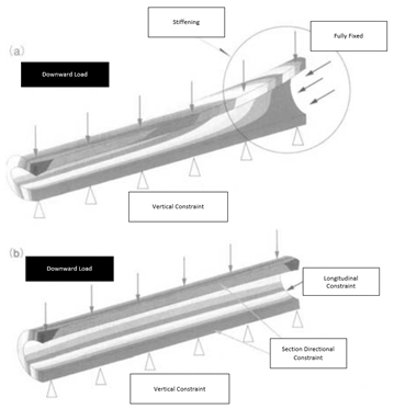
Figure 4: Example of Constraints on a Pipe: (a) When the right-end face is fully fixed, the stiffness increases there, and a large stress is generated. (b) When both faces are free, the deformation distributes evenly.
We have described different constraints extensively, but let’s now take a quick look at the some load conditions. Typical load conditions are:
One should pay particular attention to the fact that when a load is applied, as with constraints, if the force is set as applied at one point, a local stress different from the actual one is generated at that point. If this value is taken as the maximum stress value, the portion where the actual maximum stress occurs will be overlooked.
Therefore, and in conclusion, one must always doubt whether the stress generated by a constraint or load condition is the actual stress at those points. It is important to fully examine the calculated stress values, checking whether the maximums stress appears to be near the area where the boundary condition was set or whether the deformation shown is as expected under the set boundary conditions.
 |
Speaker : Gabriel Roade Category : Mechanical Software : midas MeshFree Date : 2018-10-08 |
Featured Resources
Structural Analysis
What Is Linear Static Analysis?
Read more >

Dynamic
Finite Element Analysis Types: The Ultimate Cheat Sheet
Read more >
Project Application
Boundary Conditions of Eigenvalue Analysis [IAD 4]
Read more >

Structural Analysis
The Future of Finite Element Analysis: MeshFree
Read more >
Keep Updated With Technical Contents


Keeping You Updated


![Comparison of Analysis Process [Infograph]](https://www.midasoft.com/hubfs/MIDAS%20-%20Blog/MeshFree%20-%20August%204th%20Week%20-%20Comparison%20of%20Analysis%20Process.png)