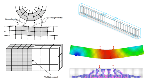
In this Intro Session our MIDAS engineer explained about Midas FEA NX's capability in simulating structural connections such as contact, wel...
5 min read
Author: JC Sun
Publish Date: 28 Dec, 2021
One of the objectives when designing structures is to prevent them from failures. Structural failure can happen when the structural elements experience stresses that are higher than their ultimate strengths. One other type of failure is buckling. Buckling is the sudden lateral deformation of the slender structure when subjected to excessive axial compressive stress. In some cases, structures fail in buckling mode before failing in compressive stresses due to the slenderness of the structural members. The phenomenon of buckling is not limited to columns. Buckling can occur in many kinds of structures and can take many forms [1]. In this article, the linear and nonlinear buckling failure of a steel bridge is investigated.
- Linear Bifurcation Buckling
Buckling may occur by bifurcation, which means that a reference configuration of the structure and an infinitesimally close (buckled) configuration are both possible at the same load [2]. The critical load {R}cr at the bifurcation can be calculated in the steps below:
First, apply the loading {R}ref to the structure, this load can be the self-weight, load from static machinery, etc. The stiffness [K]ref can be obtained and the stress stiffness matrix is [Kσ]ref. (Stress stiffness is the increase/decrease in structural stiffness caused by tensile/compressive stress, and when the structure is subjected to those conditions, its stiffness [K] gains/losses [Kσ]).
Due to the nature of the linear analysis,
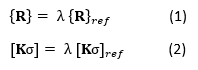
Therefore, at bifurcation point/buckling, where external loads do not change, we have the following,
Subtracting equation (3) from (4) obtains
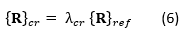
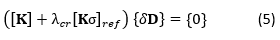 Solving the eigenvalue problem presented in equation (5) gives us the roots λcr, and choosing the smallest of λcr would give us the load factor that causes the buckling load,
- Nonlinear Buckling
A buckling problem becomes more complex when material and geometric nonlinearities are involved. Material nonlinearity happens when the material is loaded past its elastic zones, and the stress-strain curve is no longer linearly proportional. Geometric nonlinearity occurs when large deformation is involved, which is quite common in buckled structures. Geometric nonlinearity also includes boundary nonlinearity, which occurs when the contact affects the boundary conditions. Material and geometric nonlinearities often appear together, as large deformation often results in yield or crack.
In nonlinear buckling problems, a tangent stiffness [Kt] is formed, which is updated in the implicit solver at each load increment { δR }. As a limit point is approached, displacement increments will become very large [2].
However, due to the complex nature of the nonlinear analysis, one would likely fail if trying in one go. Starting with a linear model would be a good idea to troubleshoot if the analysis model contains any modeling or meshing error. Engineering judgment should also be used to see if the linear result makes sense and if the boundary conditions and loads are applied correctly. Then we can add one nonlinearity one at a time to see its effect.
- Case Study: U Frame Steel Bridge Nonlinear Buckling Analysis
Download the model file: U Frame_Update-Nonlinear Buckling.fea To look at the model, you can download Midas FEA NX here and get the 15 day free software license key here
The U frame of a steel bridge is built in Midas FEA NX. The bridge width is 9 m and the length is 35 m. The I girder flange thickness is 0.06 m and is reinforced by horizontal stiffeners every 3 m in the Y direction. The two I girders are further reinforced using lateral steel plates of 30 mm thickness every 3 m in the Y direction. Two X-bracings are added at both ends. 2D mesh is created for the plate members, and 1D frame mesh is created for the X bracing, as shown in figure 1. Also shown in figure 1 is the support boundary condition highlighted in red.
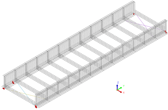
Figure 1. 2D plate mesh of the steel bridge and the 1D frame mesh of the cross bracings. The support boundary conditions are highlighted in red.
To reduce the torsional effect, displacement in Y is fixed for all the lateral plate members, as shown in Figure 2.
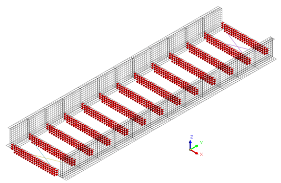
Figure 2. Lateral plates with displacement in Y fixed.
Figure 3 shows the complete mesh rendering the plate element thickness and the frame element section shape.
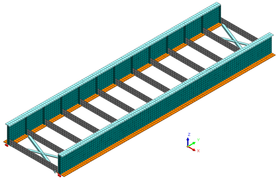
Figure 3. 2D plate mesh of the I-girder, horizontal stiffener, and the lateral support plates. 1D mesh of the X frames at the two ends with L shaped section shape.
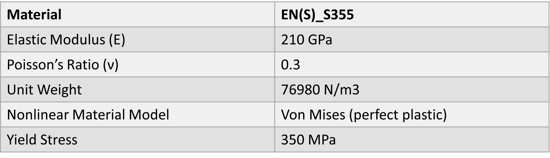
Table 1 below shows the material properties of the steel EN(S)_S355 used in this study, with its plastic behavior modeled using the perfect plastic Von Mises material model.
Table 1. Material properties of the Steel EN(S)_S355 used in this study.
- Linear Static Analysis Results
Linear static analysis is conducted initially to make sure the analysis is set up correctly and the boundary conditions and loads are applied. The maximum lateral displacement (Dx) is 163 mm in the linear static case. The result plots of lateral displacement are shown in figure 4.
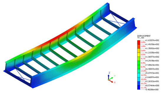
Figure 4. Lateral displacement (Dx) plot of the linear static analysis result of the bridge under self-weight. The maximum lateral displacement is 163 mm.
- Linear Buckling Analysis Results
The linear buckling modes are calculated in Midas FEA NX, and the load factors are shown as eigenvalues in table 2. λcr in equation 6 is the smallest of the positive eigenvalues, therefore the critical load factor that causes the linear bifurcation buckling of this structure is 0.962, meaning the structure will buckle under 96.2% of its self-weight. Figure 5 shows the mode shape corresponding to the buckling mode of λ=0.962.
Table 2. Eigenvalue analysis result table generated by the Midas FEA NX linear buckling analysis.
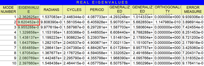
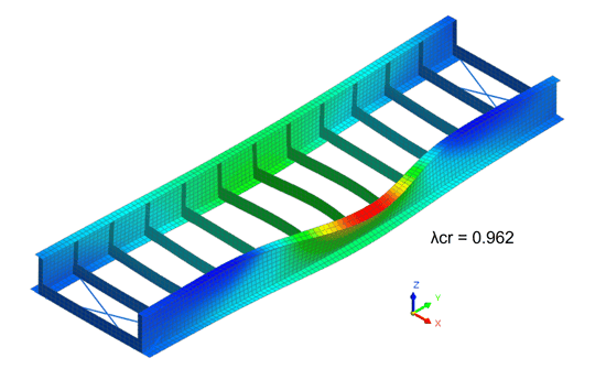
Figure 5. Modal shape corresponding to critical load factor λ=0.962.
- Nonlinear Buckling Results
Download results file plot U Frame_Update-nonlinear buckling. xlsx
We are considering material nonlinearity and geometric nonlinearity for this case. The gravity is applied incrementally in 20 segments with output at each segment, and the nonlinear static analysis is solved using the Midas FEA NX implicit full Newton-Raphson solver. In figure 6, the load factor is plotted against the maximum lateral nodal displacement (Dx). When only considering material nonlinearity, as shown in the grey curve in figure 6, the analysis stopped at a maximum load factor of 0.345 with the corresponding maximum lateral nodal displacement of 199 mm. When considering both geometric and material nonlinearity, as shown in the dotted curve, the maximum load factor of 0.293 is observed with the corresponding maximum lateral nodal displacement of 128.5 mm (interpolated).
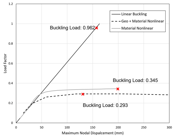
Figure 6. The plot of load factor against maximum lateral nodal displacement for the three analysis cases. The critical buckling load is highlighted in the red crosses.
- Comparison Study
The analysis result shown above shows that the bridge would buckle at self-weight. Would the structure’s resistance to buckling improve when adding more X-bracings? There are 2 X-bracings in the current model. One at each end. Another set of analyses is run on the same model with 12 X-bracings, shown in figure 7.
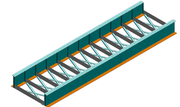
Figure 7. Modified bridge model with 12 X-bracings to study their effect on the structure's capacity in resisting buckling.
Figure 8 shows the results plot for the case of linear buckling, material nonlinearity only, and the combined effect of material and geometric nonlinearity. The buckling load for the linear static analysis improved to 1.0531, meaning that the structure can withstand its self-weight with a thin factor of safety. However, the buckling loads obtained from the two nonlinear cases have shown no significant changes.
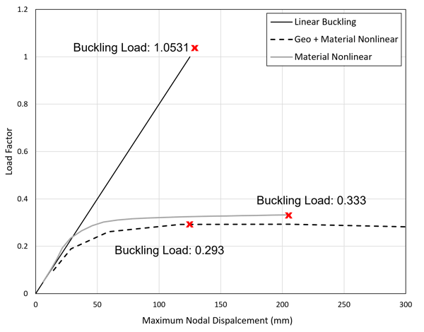
Figure 8. The plot of load factor against maximum lateral nodal displacement for the three analysis cases for the modified bridge structure. The critical buckling load is highlighted in the red crosses.
This comparison study has shown the limitation of linear analysis, which exaggerated the effect of adding the number of X-frames, which in fact did not change the nonlinear buckling load factor. The study also showed the benefit of a detailed finite element analysis tool, which can model the structural details such as the horizontal stiffeners and structural element connections.
References:
[1] Gere, James M., Goodno, Barry J. Mechanics of Materials, Seventh Edition, Cengage Learning, 2009, Toronto, ON.
[2] Cook, Robert D., Malkus, David S., Plesha, Michael E., Witt, Robert J., Concepts and Applications of Finite Element Analysis, Fourth Edition, 2001, John Wiley & Sons Inc., New York, NY.
https://www.midasoft.com/bridge-library/civil/products/midasfeanx
jsun@midasoft.com
Add a Comment