Expert Tips: Iteration and Optimization 2

Iteration and Optimization

Iteration is just a repeated calculation.

If we want to solve an equation x + 1 = 5 , we can assume x and check whether x + 1 = 5 or not. If not, we can try another value of x and repeat this calculation until x + 1 = 5.

In this simple equation, we can solve x = 5 - 1 = 4 easily. But some engineering problems are more complicated and iteration is more efficient and/or sometimes iteration is the only way to find the solution.

If we want to solve another equation xy = 5, this is rather complicated because there are infinite combinations of x and y’s. However, if we can add some “constraints” like we want to minimize x + y, we can find the solution and this is called the “optimization problem”.

(If another condition is something like, x + y = 4, this is not an optimization problem because there is only one set of solutions.)

In our pile cap problems, there are many combinations of pile cap dimensions that satisfy all requirements. In this case, we can try to find the pile cap dimensions that satisfy all requirements and corresponds to the minimum volume, and this is a good example of both “Iteration” and “Optimization”.

(There can be an argument that the minimum volume can not be optimum. Someone can insist that the optimum shall be minimum cost and we have to consider reinforcements, forwork, etc. The author has no objection to this, but still believes minimum volume is a good choice as the target.)

“Optimization” does need “Iteration” and the purpose of “Iteration” is “Optimization”, so these two terminologies are somewhat mixed and have different meanings for each engineer. It is not a universal/correct definition, but the author accepts “Iteration” as checks for all possible scenarios, and “Optimization” as finding only the optimum in the fastest way.

Iteration

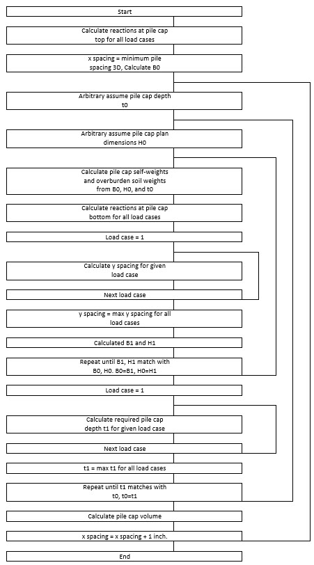
The following flow chart shows how to find the minimum pile cap dimensions by “Iteration”. As can be seen, the calculation is just a repetition. We do need voluminous calculations but we have no problems because we have computers.

Once upon a time, the main focus was to make the calculation procedure as efficient as possible to save computer time, but now this approach has little meaning and the importance is to make the procedure as simple/easy as possible for us, humans.

Optimization

We have another approach to solve these problems called “Optimization”.

Again, if we want to solve an equation x + 1 = 5, first we can assume x = 1 and calculated x + 1, now we know that x can not be 1 and we try another value of x based on the previous calculation that x is not 1.

In the “Iteration”, we try the next value of x as somewhat arbitrary as 1,2,3,… but in the “Optimization” there is a very refined way to select the next trial value of x, so we can find the solution very rapidly. Like other fields of engineering, the development of “Optimization” is just dramatic.

Going back to our pile cap problems, we can ask the computer to find x spacing and y spacing that satisfy all requirements and produce the minimum volume, and the computer can find these numbers very easily.

Looks perfect.

But there are always pros and cons.

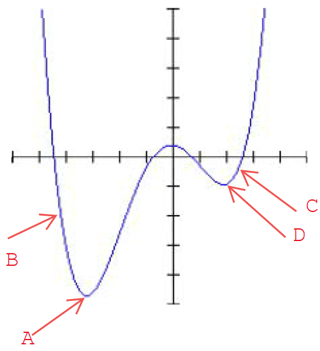
Say we are finding the minimum point A.

In the “Optimization”, first we or the computer arbitrarily select a point “B” and calculate the slopes at just left of B and at just right of B, then the computer knows the right side is downward and selects the next trial value somewhere at the right side. The actual calculation is much more complex and the computer can find point A very rapidly.

But, if we or the computer selects point C as a trial point, the computer can find point D as the minimum point instead of the real minimum point A.

Our problem is rather a simple one and we may not worry about this problem, but in the more complex problems, we have to check whether the output is the real optimum or not. But the problem, “how to check” remains in many cases.

The other problem occurs in the case where the curve is rather flat near the minimum locations. The computer can not find the exact minimum point, rather can find a point close to the minimum point within the allowable error.

In our example, the pile cap volume is close to the minimum in the range of x spacing between 5’-0” to 6’-6”. Strictly speaking, all we know is the solution “may” be somewhere around 5’-8” location.

Closure

Engineering judgment and past experiences from our fore-engineers shall not be underestimated. In the same sense, we do not need to assume our guess is the “optimum”. Now we have computers and we can confirm our engineering judgment and past experiences very easily.

The author prefers simple “Iteration” because it is easy and there is no missing spot. The computation time is longer but acceptable in most real-world problems.

I heard some persons use Excel just as a word processor and even never use the sum function, rather he/she calculates the summation by calculators and input the calculated value to the cell. I am not blaming or laughing at him/her. He/she should have used calculators for a long time and very confident with the results, but for any reason, not that comfortable with Excel’s function.

“Iteration” and/or “Optimization” are not the only or the perfect way for our design, but they are one of the best ways and worth trying.

Numerical Example

A practical approach to finding the optimum pile arrangement by “Iteration” will be discussed. We have two variables to define a pile cap. One is pile spacing, either x-direction or y-direction, and the other one is pile cap thickness. The purpose of this iteration is to find these two values that produce the minimum pile cap volume.

In most cases, the definition of “Optimum” itself is not clear. In this discussion, we assume that minimum pile cap volume corresponds to the “Optimum” design.

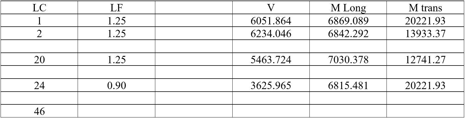
Assume we have a total of 46 load cases.

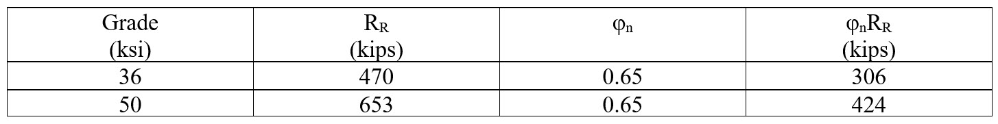
Try H14×89, 50 ksi piles.

Step 1) Calculate reactions at footing top

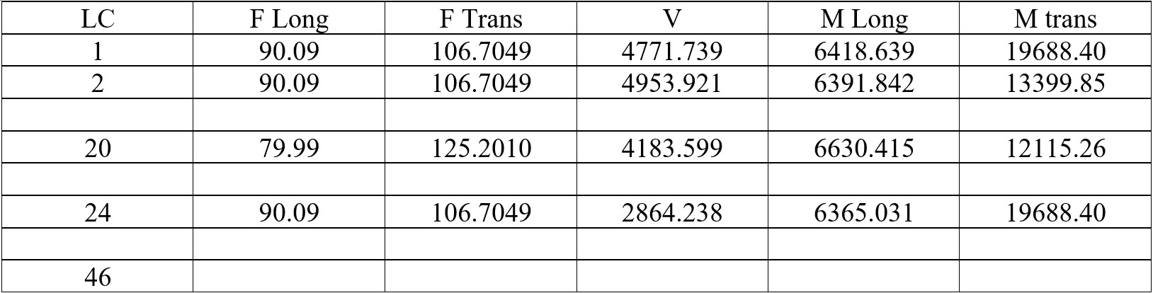
Vu max = 4954 kips and we need more than (4954kips)/(424kips/EA) = 12 EA piles whatever we do.

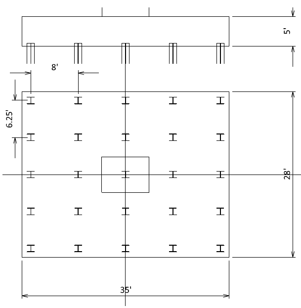
Try 5 × 5 = 25 EA pile arrangement.

Step 2) Try x sps = 8 ft

B = (5EA – 1)(8ft) + 2(1.5ft) = 35 ft

Step 3) Try pile cap thickness = 5 ft

Step 4) Try H = 28 ft

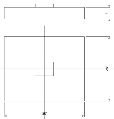
Step5) Calculate pile cap and soil weights

W = (35’)(28’){(0.150ckf)(5’) + (0.100kcf)(2’)} = 931 kips

Step6) Calculate reactions at footing bottom

Calculations are shown for load case 24

Pu = 3025 + (1/1.1)(0.90)(931) = 3786 kips

Mu Long = 6365 + (5’)(90.09) = 6815 ft-kips

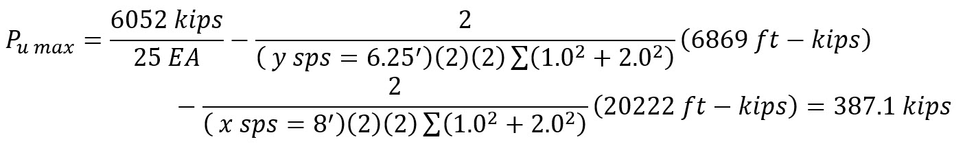
Mu Trans = 19688 + (5’)(106.7) + 17123 = 20222 ft-kips

Step 7) calculate y sps which limits maximum pile reaction would be less than pile capacity 424 kips.

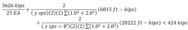
y sps > 1.533 ft

Step 8) Calculate y sps which prohibits pile uplifts.

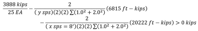
y sps > 6.206 ft                                                                                                             Controls

Repeat Step7) and Step8) for all load cases.

Select y sps = 6.250 ft

Step 9) Calculate H

H = (5EA – 1)(6.25ft) + 2(1.5ft) = 28 ft

Repeat Step4) to Step9) until assumed H matches with calculated H

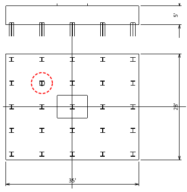
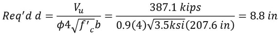
Step 10) Punching shear check for single pile

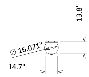
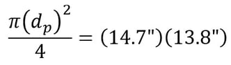
dp = 16.07 in

Maximum pile reaction (load case 1)

d = t – 10” = 4’-2”

b = π{dp + 2(d/2)} = π{(16.07” + 2(50”/2)) = 207.6 in

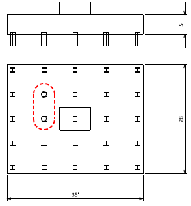
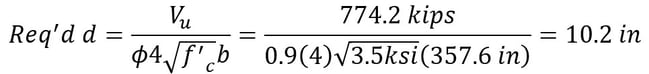
Step 11) Punching shear check for two piles

Pu max = (2)(387.1kips) = 774.2 kips (conservative)

b = 207.6 in + (2EA)Min(8’, 6.25’) = 357.6 in

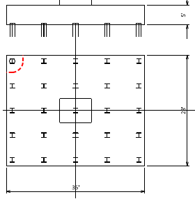
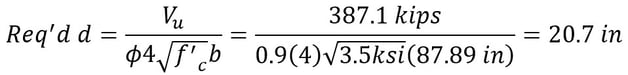
Step 12) Punching shear check for corner pile

b = (207.6in / 4) + (2EA)(1.5’) = 87.89 in

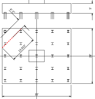
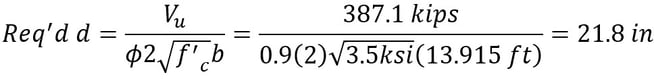
Step 13) One-way shear check at d (or 13 in) from the face of the corner pile

b = 13.915 ft

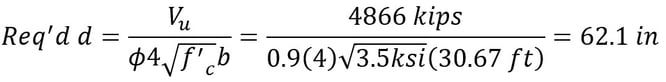
Step 14) Two-way punching shear check

Load case 2 controls.

Vu = (6234 kips)(24 EA/25 EA) –{(35’)(38’) - (8’ + 50”)(6’ + 50”)}{(0.150ckf)(5’) + (0.100kcf)(2’)} = 5985 – 1119 = 4866 kips

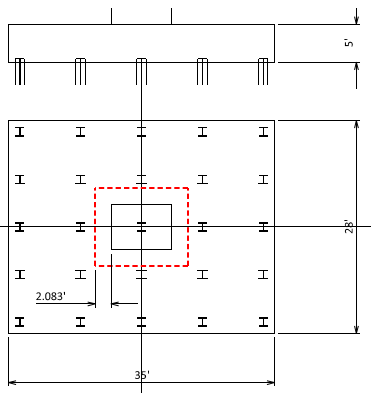
b = 8’ + 6’ + 8(50”/2) = 30.67 ft

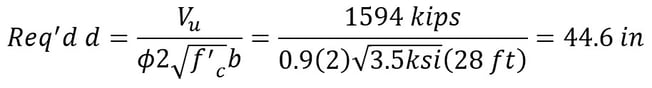
Step 15) Transverse one-way shear check

Check dv from the column face

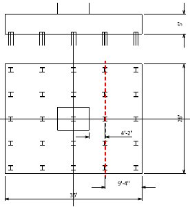
Vu = (5EA)(387.1kips) – 1.25(28’)(9’-4”){(0.150ckf)(5’) + (0.100kcf)(2’)} = 1936 – 341.1 = 1594 kips

b = 28 ft

Step 16) Longitudinal one-way shear check

Check dv from the column face

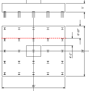
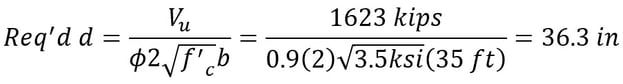
Vu = (5EA)(387.1kips) – 1.1(1.25)(35’)(6’-10”){(0.150ckf)(5’) + (0.100kcf)(2’)} = 1936 – 312.4 = 1623 kips

b = 35 ft

Required t min = 62.1 in + 10 in = 72.1 in = 6’-3” > Assumed t = 5’-0”

N.G.

Repeat Step3) to Step15).

Editor: Edgar De Los Santos

e.santos@midasoft.com