The bridge load rating is a procedure to evaluate the adequacy of various structural components to carry predetermined live loads. In simple...
5 min read
Author: Ethan Baker P.E., S.E.
Publish Date: 17 Apr, 2024
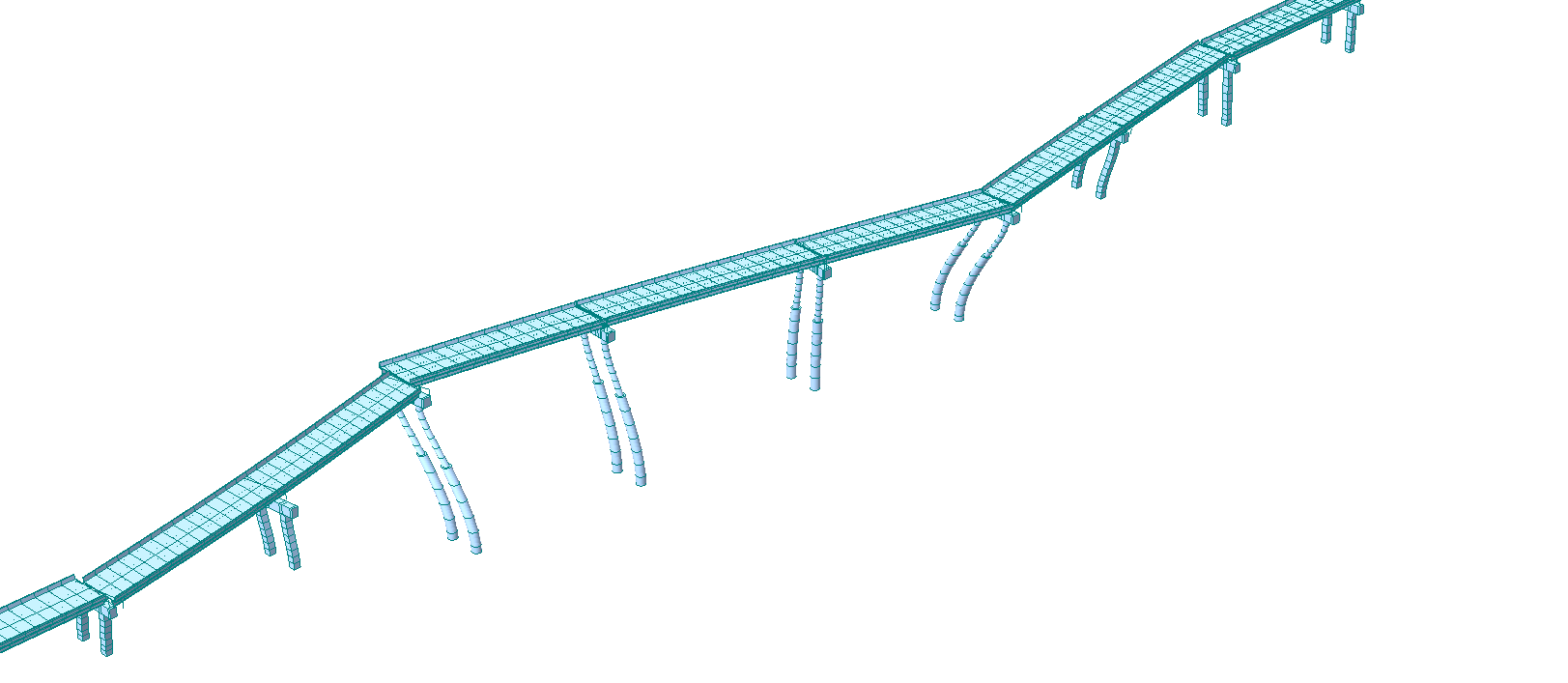
Introduction:In the world of bridge design, seismic analysis is sometimes seen as a rigorous process that can yield results that, at first, are not intuitive. The AASHTO LRFD Bridge Design Specifications require different analysis methods depending on seismic performance zone, bridge operational classification, and structural regularity. Each type of seismic analysis can vary in level of complexity. With more powerful analysis methods and complexity possible where software is employed, it is important to verify that the analysis output is reasonable. This article outlines some simple, but powerful, hand-calculations and model verification checks that can be performed to validate a seismic analysis model. |
Seismic Mass
From single-mode analysis to non-linear time history analysis, seismic mass is one of the most important factors in a representative model as it directly influences the dynamic behavior of the structure. When subjected to ground motion during an earthquake, the mass of the structure interacts with acceleration to create inertial forces. Underestimation of the mass can lead to inaccurate design forces and displacements. Mass also plays a key role in determining the structure’s modes of vibration. An accurate accounting of contributing seismic mass ensures reliable mode shapes and frequencies, which directly impact the structure’s seismic response.
Also of importance is the distribution of mass. Rather than modeling lengthy elements, elements should thoughtfully be discretized to ensure their masses, which are lumped to the connecting nodes, are well distributed. However, too much discretization can lead to unnecessary modes. A balanced approach is recommended, and the results should be limited to several contributing modes.
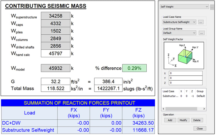
A quick hand calculation of the contributing seismic mass, including the weight of the deck, girders, railing, diaphragms/cross-frames, stay-in-place formwork, sidewalks, etc. can easily be compared with the output from the analysis. Large differences in hand-calculated mass vs. modeled mass could indicate issues with geometric inputs, material weight density, or possibly issues communicating to the model to consider the weight of structural components as part of the overall mass.
Fig 1. Top Left – Hand-calculated contributing seismic mass. Bottom Left – midas Civil reaction forces output. Right – midas Civil Self Weight Loads to Masses operation.
Stiffness
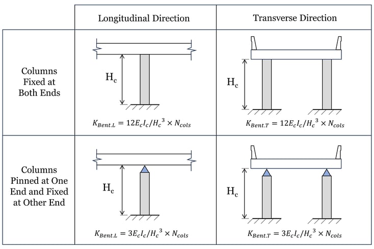
The lateral stiffness of a column within a substructure system can be estimated as 3EI/L3 (fixed-pinned or fixed-free) or 12EI/L3 (fixed-fixed) depending on the substructure boundary conditions for the given direction of loading. An equivalent stiffness could also be calculated for the system by considering the stiffness contribution of the foundation elements and bearings.
The effective stiffness of the modeled substructure can be determined by applying a unit force to the top of the substructure system and dividing by the resultant deflection. A large difference in hand-calculated stiffness values vs. modeled stiffnesses could indicate issues with section properties, material properties, or boundary conditions. Superstructure axial and flexural stiffnesses also play a role in the global stiffness of the structure, but they are usually relatively stiff enough to be considered rigid for hand-calculation purposes.
Figure 2. Lateral stiffness estimation of substructure systems. Note that substructure systems may be best represented with differing boundary conditions for each direction (i.e. pinned-fixed columns in the longitudinal direction and fixed-fixed columns in the transverse direction).
Period, Frequencies, & Mode Shapes
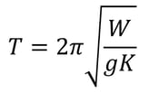
Once mass and stiffness are calculated, a quick calculation of the fundamental period for each direction of a single-degree-of-freedom system can be performed using the equation below:
where T is the fundamental period, W is the total contributing weight of the structure, g is the acceleration due to gravity, and K is the lateral stiffness of the system.
A large difference between calculated fundamental periods and periods resulting from the analysis (usually the first few modes) could indicate issues with mass or stiffness. This could be due to incorrect material property or boundary conditions input.
It is important to reflect on the fundamentals of structural dynamics and engineering judgment as well: Is the bridge stiffer in the transverse direction or the longitudinal direction? Do the mode shapes and frequencies/periods reflect what you would expect?
Displacements
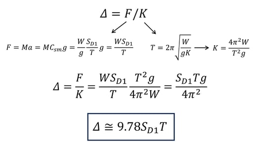
Some simplifying assumptions can be made to estimate the displacement of the bridge due to seismic loading. Assuming a single-degree-of-freedom system, Hooke’s law can be applied. From there, equations for force and stiffness can be determined from Newton’s Second Law of Motion and the equation for the period shown above, respectively. The equations below assume a fundamental period that is greater than TS (the corner period at which the acceleration response spectrum changes from being independent of the period to being inversely proportional to the period) and a damping ratio of 5%. Note this is an oversimplification of the analysis, and there may be more variation observed in displacements of complex systems with large deviations of stiffness between components.
Figure 3. Derivation of oversimplified equation for displacement due to seismic loads where Δ is displacement, F is force, M is seismic mass, a is acceleration, Csm is the elastic seismic response coefficient for the considered mode, and SD1 is the horizontal response spectral acceleration coefficient at 1.0s period modified by the long-period site factor (see above for definitions of all other variables). Equations assume a fundamental period greater than TS and a damping ratio of 5%.
Modal Mass Participation, Base Shear, & Load Path
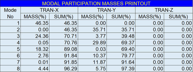
Verify that the modal mass participation (Mass%) from the eigenvalue analysis is ≥ 90% for both primary directions. In midas Civil, this can be found in the Results - Results Tables - Vibration Mode Shape table under the heading “Model Participation Masses Printout.”
Figure 4. An example of a modal mass participation output from midas Civil.
AASHTO LRFD Bridge Design Specifications Article 4.7.4.3.3 states that member forces and displacements may be estimated by combining the response quantities from individual modes by the Complete Quadratic Combination (CQC) method. The Square-Root-of-the-Sum-of-the-Squares (SRSS) method is simple enough to perform by hand and can be used as a double check of analysis results. The SRSS hand-calculated base shear values should compare relatively well with the CQC base shear values from the analysis when the modes are well-spaced.
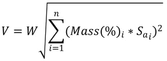
Base shear (V) using the SRSS method can be calculated with the following equation:
where i is a given mode, n is the number of modes considered, and Sa is the mode’s corresponding design acceleration (see above for definitions of all other variables).
It is important to observe the analysis results to verify that the load path makes sense and that the mode shapes with the most mass participation are reasonable. Substructure units can be investigated to verify that stiffer bents generally attract more force and that reactions at the boundary conditions are reasonable for the structural configuration. Displacement output can be invaluable in troubleshooting instabilities within the model, verifying fixity between elements, and checking for unreasonable responses such as elements moving past each other or unexpected displacement at boundary conditions.
Utilize Simpler Analysis Methods
If more complex analysis results are still in question, a quick Single-Mode Spectral Analysis or Uniform Load Method Analysis can be performed manually for comparison. A simple frame analysis model, with springs representing the stiffness of each bent, could be used. AASHTO LRFD Bridge Design Specifications Articles C4.7.4.3.2b and C4.7.4.3.2c outline steps for the Single-Mode Spectral Method and the Uniform Load Method, respectively. Note that the Single-Mode Spectral Method may be more accurate when most of the mass participation is within the first mode for the given direction.
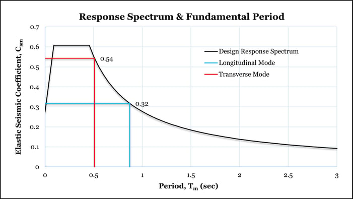
Figure 5. Design response spectrum plotted with longitudinal and transverse periods determined from a Single-Mode Spectral Analysis.
Final Thoughts & Conclusion
With any modeling, it may be best to “start small.” Begin with hand calculations considering a simplification of the bridge model. For example, assume fixed-base columns rather than considering soil-structure interaction effects right away. Once the model is built and the simplified iteration results make sense, incrementally build in the necessary complexity.
It is critical to verify that analysis results are reasonable. Mass and stiffness inputs, fundamental period, displacement, and base shear results can be validated through hand calculations using simplified equations. Additionally, the model results can be observed to verify that the load path, displacements, reactions, mass participation, and other outputs seem realistic. In the world of structural engineering, computer output is only useful if it can be correctly interpreted and verified for reasonableness.
Sources:
- AASHTO LRFD Bridge Design Specifications. American Association of State Highway and Transportation Officials, 9th Edition, 2020.
- LRFD Seismic Analysis and Design of Bridges Reference Manual. U.S. Department of Transportation, Federal Highway Administration, National Highway Institute, FHWA-NHI-15-004, October 2014.
Add a Comment