Expert Tip: Determining Concurrent Live Load for Strut and Tie Models

In the article "strut-and-tie modeling for pier caps", we have discussed the definition of strut-and-tie analysis and how to construct a strut-and-tie model using the example of pier cap. After creating the geometry of a strut-and-tie model, the next step usually is calculating dead and live loads from the superstructure. This article discusses how to determine the boundary loads for a pier cap with a superstructure that has irregular geometries. 

• What is Lever Rule? 

Applying the lever rule allows us to consider the deck to be simply supported between girder lines in the transverse direction. We can then use a line girder analysis to determine the tributary length for loads on each supported superstructure span, and use different live load placements that maximize these reaction force (shear and moment) from the deck at the girders following the AASHTO rules for lane width, vehicle placement, and multiple presence provisions. 

• Is Lever Rule Always Able to Obtain Superstructure Dead and Live Load? 

However, there are cases where lever rule cannot be applied. Figure 1 shows a bridge with a significant skew, and with a girder line that stops at the top of a pier, and with cross frames that are oriented at a different angle than the piers, and with different span lengths. Using lever rule in this case would not be accurate to determine what the superstructure reaction should be that is applied to the pier cap. Therefore, we included the superstructure model and the piers in the same analysis model and used the superstructure model to determine what the bearing loads should be. For this analysis to be accurate, all the live load forces for each of the different cases need to be concurrent with one another, and we cannot use a live load envelope. This article shows the process of determining the concurrent live loads using midas Civil to find the load cases that maximizes the shear and moment reactions at the pier cap. 

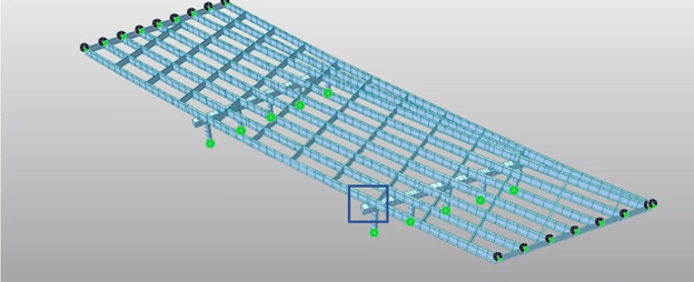
Figure 1. Skewed steel girder bridge with sub beam and variable girder span lengths.

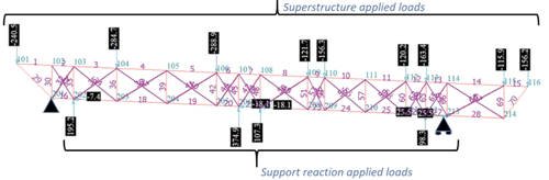
Figure 2 shows the zoomed view of the region highlighted in blue box from figure 1. What we are trying to do is to figure out what would be the live load from the superstructure that maximizes the vertical shear and negative moment at the element that is highlighted by the blue box. We can define that as an equivalent static load case so that we can be sure its loads are concurrent. In this example, we are interested in obtaining the maximum HL-93 shear and negative moment in the element 30053 part i, shown in figure 3. 

Figure 2. Maximum HL-93 Shear and negative moment in element 30053 [i]

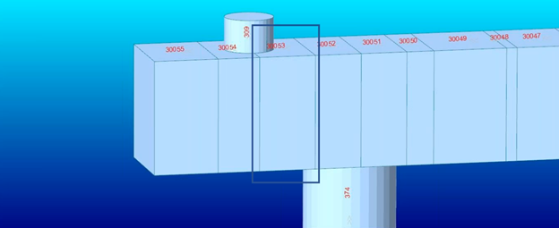
Figure 3. Maximum HL-93 Shear and negative moment in element 30053 [i]

To determine which live load maximizes the loading conditions at element 30053i, the following steps can be followed. As shown in figure 4, in midas Civil post-processor, we can select all the individual load patterns, and select element of interest (30053i). After requesting the list of forces at the element 30053i, we can visually determine which of the live load pattern that maximizes the forces at element 30053i, as shown in figure 5. 

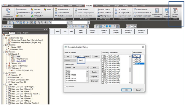
Figure 4. Results -> Tables -> Results Tables -> Records Activation Dialog.

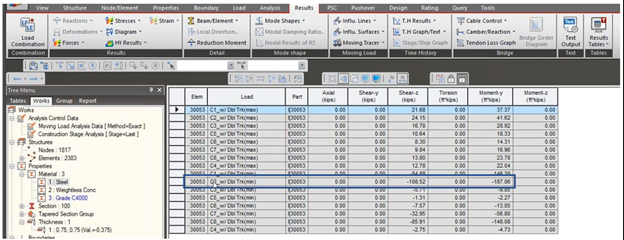
Figure 5. Case 2 live load pattern that could maximize the loading conditions at the element 30035 [i].

After determining the load pattern that maximizes the loading conditions at element 30053i (load pattern: C2_w/Dbl Trk_min), we can visualize this load pattern and save it as an equivalent static load. To visualize this load pattern: Results -> Moving Load -> Moving Tracer, would show us the position of the vehicle that contribute to the load which maximizes the shear and vertical moments at the element of interest, as shown in figure 6. 

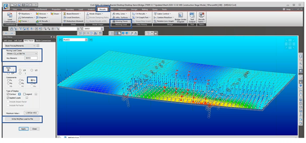
Figure 6. Moving load tracer for load case C2_w/Dbi Trk that contributes to the maximum loads at element 30035.

To define this load pattern as an equivalent static load case for strut-and-tie analysis, follow the highlighted blue boxes in figure 6 and click "Write Min/Max Load to File", we can get a text-based file (.mct file) shown in figure7. 

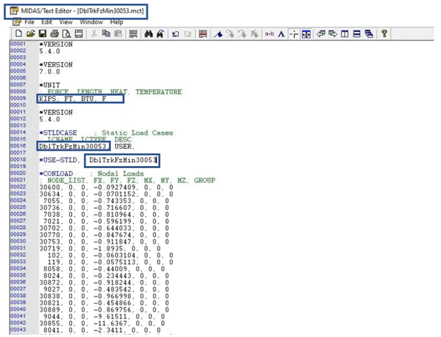
Figure 7. Midas Civil .mct file that specifies the static load representing the truck location that contributes to the maximum loading effect at the element 30035.

After saving this .mct file, you can go to Tools - MCT Command Shell -> Open to open the above saved .mct file and hit "run". This would create a static load case shown in figure 8, and by adding this equivalent static live load case, we can get the concurrent loads for our strut-and-tie model.   

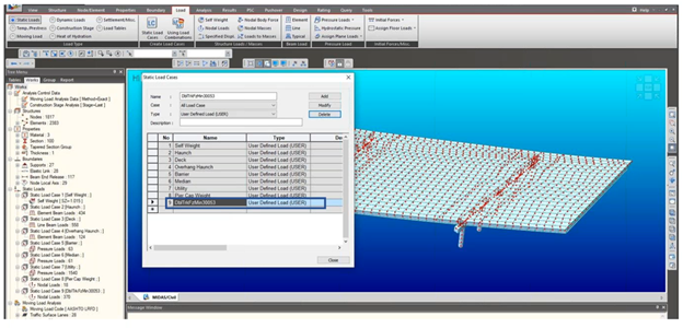
Figure 8. Equivalent static load case created from moving load tracer.

Editor: JC Sun

jsun@midasoft.com