Expert Tip: Suspension Bridges 2

4th-order differential equation

Eq(2) is a 4th-order differential equation, and we can imagine it is not simple to solve.

Fig 8 Leon Moisseiff 1872-1943

Moisseiff solved Melan’s equation in his 20s, and his elegant solution is as follows.

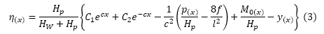
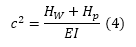
In eq(3), C1 and C2 are integral constants, Mo(x) is the moment as a simple span for the given loading p(x), y(x) is cable coordinates from the pylon top, and c is defined as follows.

From eq(3), we can get girder moment, girder shear, and girder uplift force easily through differentiation as follows.

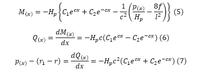
In eq(7), the term –(r1-r) is the uplift force from hangers and if we know these forces, we can analyze the girder as a simple beam with loadings p(x) and –(r1-r). As can be seen, –(r1-r) is also dependent to Hp, which is function of live load p(x), we do need iteration.

In eq(3), the term Hp in the right side is still unknown, and we need another equation, called cable equation.

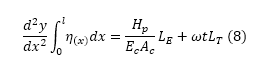
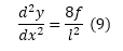
In eq(8), EcAc is the axial stiffness of the cable, w is the coefficient of cable thermal expansion, t is temperature change (rise is assumed positive), and d2y/dx2 is determined from cable geometry as follows.

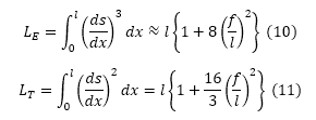
LE and LT are also defined from the cable geometry as follows.

Substitute eq(3),(9) into eq(8), we can get,

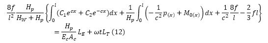
Eq(12) is a non-linear equation, and we need iteration to solve it. However, the convergence is rapid, and we have no problem solving with computers. In the real calculation, we need only a couple of times iterations.

Moisseiff"s solution shown for a loading case

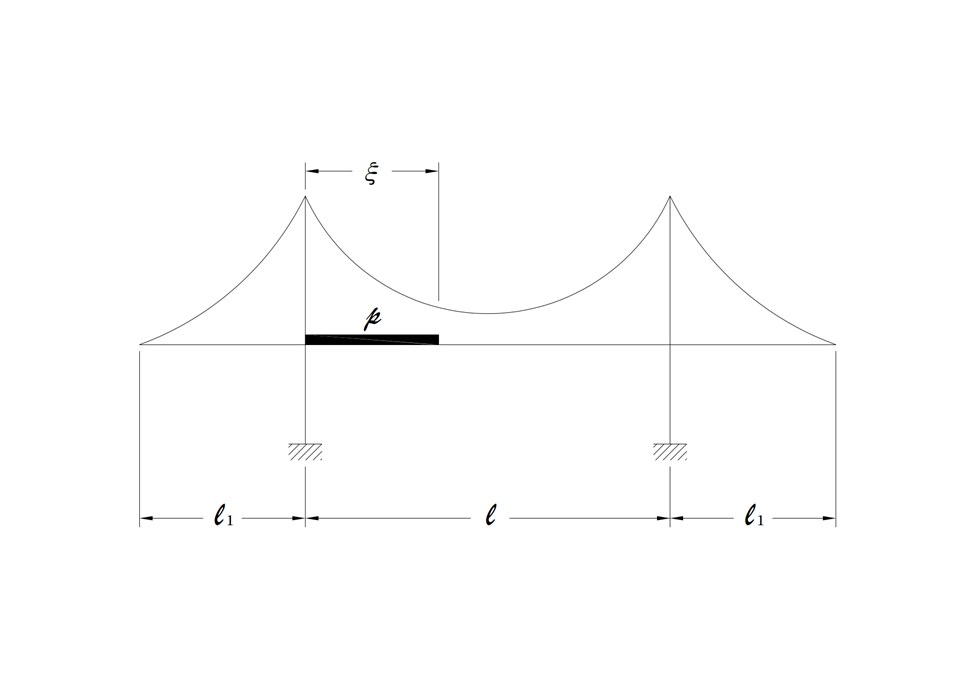
Fig 9 Constant load p(x)=p from x=0 to x=ξ in the center span with temperature rise

As an example, a detailed solution from Moisseiff is shown for a loading case shown in Fig 9. p(x)=p for 0≤x≤ξ and p(x)=0 for ξ≤x≤L.

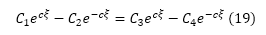
From eq(3), the deflection equations are

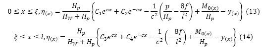
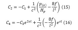
At x=0 and x=L, deflection η(x)=0, cable coordinates from pylon top y(x)=0, and moments as a simple beam M0(x)=0. From these conditions,

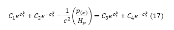
The deflection η(x=ξ) shall be identical both from eq(13) and eq(14).

The equation for curvature can be derived from eq(3) through differentiation.

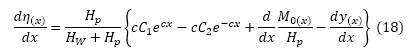
The curvature dη(x=ξ)/dx shall be identical at x=ξ.

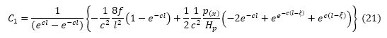
From eq(17) and eq(19),

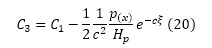
Substitute eq(15),(16) into eq(17),(19),

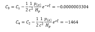
For side spans, since no loads are applied, p(x)=0 and M0(x)=0. Through the same methods, we can find integral constants as follows.

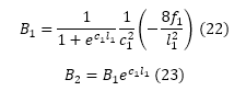
In eq(22),(23), subscript 1 represents these integral constants B1 and B2 for side spans.

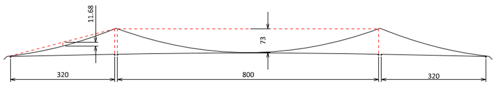
Fig 10 Example bridge from Hirai

Let’s try to find the maximum moment at x=kL=0.2L=160m at the center span.

Design conditions are as follows.

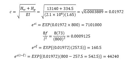
First, we have to find out the loaded length ξL. We are trying to find out the maximum moment at kL=0.2L=160m, and we need a loaded length ξL that results in the maximum moment at this location, which is unknown. Melan’s equation is a non-linear equation, and the principle of superposition cannot be applied. This means we cannot apply influence line analysis. How to find out the loaded length ξL? One method is iteration. Assume the loaded length ξL and calculate the moments. Adjust ξL until we get the maximum moments. This is a kind of simple optimization, and we do not have any problem with computers (Moisseiff did it only by slide rules!).

Assume ξL=(0.3219)(800m)=257.5m

We do not know Hp, and we need another iteration.

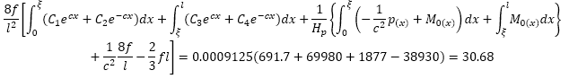
Assume Hp = 334.5 kips, for the center span

For loaded portion 0≤x≤ξ,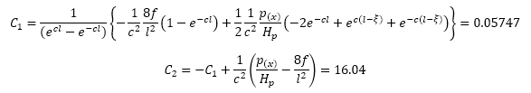

For unloaded portion ξ≤x≤L,

Cable equation for center span

For side span

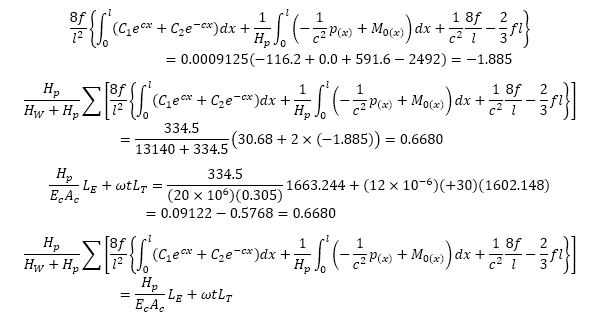
Assumed Hp=334.5 kips satisfies this equation. Otherwise, we need to update Hp and perform the same calculations. There are some methods to update Hp to accelerate convergency. However, it has little meaning now with computers and will not be discussed.

With Hp, the moment at x=kL=160m can be calculated as follows.

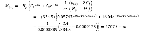
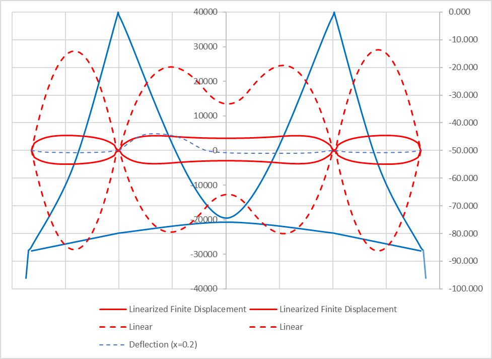
Fig 11 Girder moment due to live load

In Fig 11, the blue dashed line shows girder moments due to live load, which results in the maximum moment at x=kL=160m. As can be seen, it matches very well with the results of non-linear FEM results.

From eq(7), we can calculate the hanger uplift force as shown below.

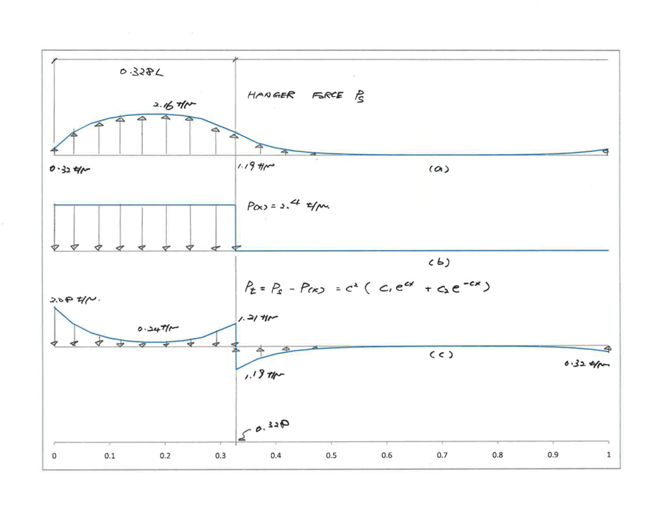
Fig12 Hanger force Ps, applied load p(x), net hanger force Pt

With the load Pt, we can calculate girder moment, shear, and deflection as an 800m span simple beam.

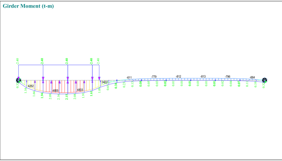
Fig 13 Girder moment as a simple beam with loading Pt

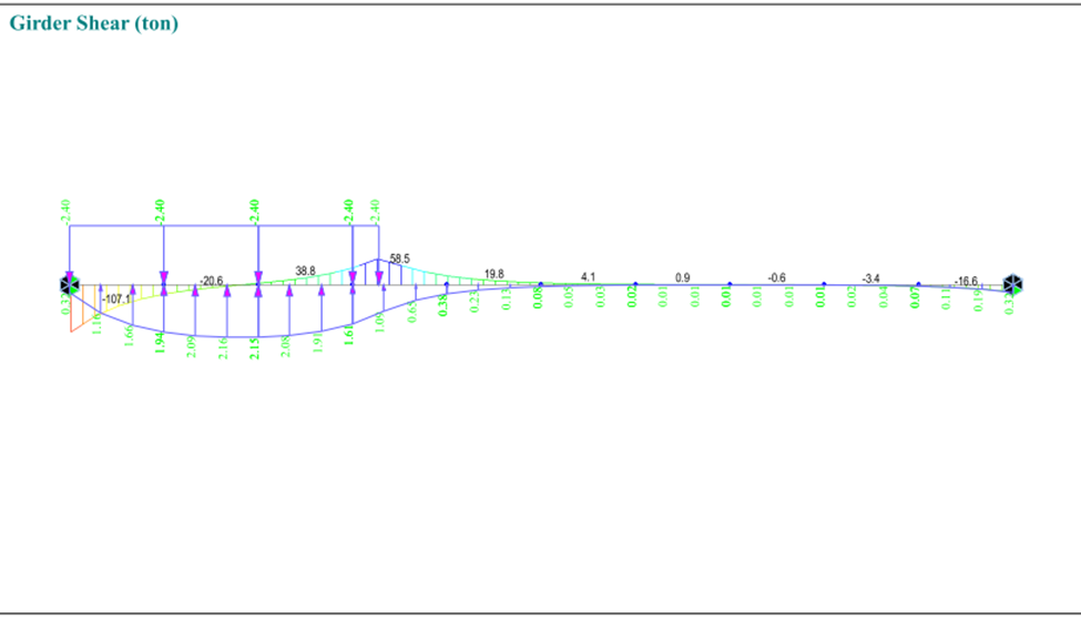
Fig 14 Girder shear as a simple beam with loading Pt

Fig 15 Girder shear as a simple beam with loading Pt

From Fig 13, the maximum moment at x=kL=160m is around 4833 t-m which is 103% of 4707 t-m. These minor differences are due to the simplification of the loadings. The actual loading is an exponential function but was simplified as a linear function. We can increase the accuracy easily with more loading divisions.