Expert Tip: Suspension Bridges 1

The Question

We have structural analysis programs. Can we make the model (like other conventional bridges) and perform the analysis (as usual)?

The Answer

The short answer is yes, we can! 

But the results may be useless. The scary parts of FEM are it gives results without any warning/error message, but the output may not be correct or useless.

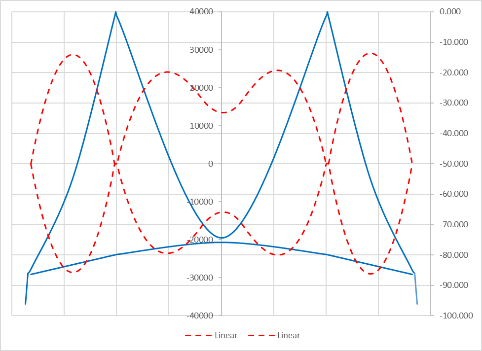
Fig1 Girder moments due to live load from linear/conventional analysis

Fig1 shows girder moments due to live loads for a medium-span suspension bridge. The main span is around 2600 ft (now the longest one was built by Turkish engineers, and the main span, between pylon to pylon, is 6600ft, much more than a mile!). This example bridge is not a real one and was proposed by Dr. Hirai for comparison (Steel Bridge III, by Hiral Atsushi).

We can analyze suspension bridges in a conventional way. However, the output moment is too big, and we cannot design the section. From conventional linear analysis (dashed line), we got a moment around 29,000 t-m at the center of the side span. Moment 29,000 t-m is huge and not easy to design for this moment. This is one of the main reasons why we couldn’t design a long-span suspension bridge in the 19^th century, and the span limit was around 2,000 ft.

Fig2 John A. Roebling suspension bridge, opened 1867, main span 1057 ft (https://en.wikipedia.org/wiki/John_A._Roebling_Suspension_Bridge)

If you have hawk’s eyes, you can see that the girders are somewhat stocky for these traditional suspension bridges in the 19^th century.

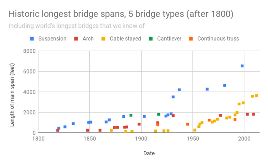
Fig3. Historic longest bridge spans (https://aiimpacts.org/historic-trends-in-bridge-span-length/)

As can be seen from Fig3, somewhere in the 1930s, the bridge span went up dramatically, approximately twice. What has happened in these eras?

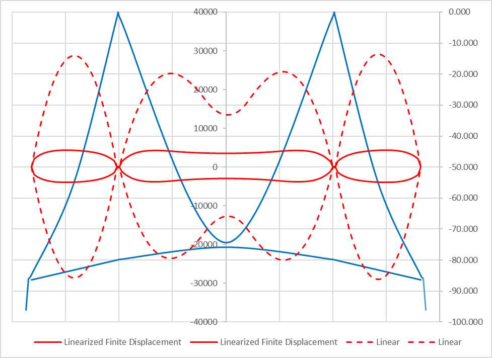
Fig4 Girder moments due to live load from linear/conventional and linearized finite displacement analysis

If we consider some kinds of non-linearity (red solid line), even a very simple one like linearized finite displacement methods, the moment will drop down to 4,300 t-m, and we are much more comfortable designing the girder section.

How is this possible?

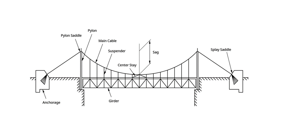
Fig5 Suspension bridge concept (from midasBridge)

From the point of a girder’s view, a suspension bridge is nothing more than a simple girder that is supported by main cable, through hangers (some modern or railway suspension bridges have continuous girders, but most suspension bridges have expansion joints at the pylon and can be considered as simple spans. Sometimes these suspension bridges are called three-span, two-hinge suspension bridges, very typical ones).

In suspension bridges, the girders are supported by three main components.

1. Axial (vertical) stiffness of hangers
2. Transverse (vertical) stiffness of main cables, and
3. Flexural (horizontal) stiffness of pylons.

    

   Comparing the transverse (vertical) stiffness of main cables, the axial (vertical) stiffness of hangers is too big, and we can consider the hanger as inextensible membranes (sometimes the theory of suspension bridge analysis is called stiff membrane theory).

On the other hand, the flexure (horizontal) stiffness of the pylon is too small compared to the longitudinal (horizontal) stiffness of the main cables, and we can ignore the flexure (horizontal) stiffness of the pylon and just consider the cables are simply supported at the pylon top.

Now we know that the girders are supported mainly by the transverse (vertical) stiffness from the main cable.

If we consider cables as truss elements, we know that truss elements have only axial stiffness EA/L and no transverse stiffnesses. In other words, we have to design the girders something similar to simple spans. Even though there are some contributions from the geometric cable inclination, designing a 2,600 ft simple girder is not an easy task.

However, if the truss elements have any axial force, the stiffness matrix is somewhat different.

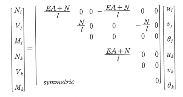
Fig6 Element stiffness for truss elements with axial force, (Planning and analysis of suspension bridges, by S. Lee)

The axial stiffness is (EA+N)/L, where N is the axial force. Compared to EA, the effect of N is small, and we can ignore N in the axial direction. But in the transverse direction, there is no stiffness (i.e., unstable) in the pure truss element, but now we have stiffness N/L considering the axial force. The stiffness increase from zero to N/L is critical in the suspension bridge analysis and the theoretical base for designing a long-span suspension bridge.

An example

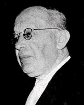
Fig7 Josef Melan 1853-1941 (https://www.usti-aussig.net/de/autori/karta/jmeno/17-josef-melan)

In 1888, a brilliant Austrian engineer Josef Melan pointed out that we have to consider these effects to design a long-span suspension bridge (Melan, J., Theorie der eisernen Bogenbrücken und der Hängebrücken, 2^nd ed., 1888). He derived a formula for girder moments due to live loads as eq(1).

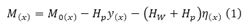
In eq(1), M(x) is girder moment due to “live” load, Hw and Hp are cable tension due to “dead” and live load, η(x) is girder deflection, y(x) is the cable geometry. Melan is the first one who pointed out that the girder moment due to the “live” load can be reduced if we consider the “dead” load effects in the cable. For conventional bridges, we can analyze live load effects without considering dead loads. In other words, we can consider the dead load effects and live load effects separately and then combine these results together. In the suspension bridge analysis, we must consider the dead load effects when we analyze the live load effects.

This methodology is a kind of non-linear analysis and is sometimes called deflection theory, 2^nd order theory, finite displacement theory, etc. Unlike conventional linear theory, each theory has some differences and gives different results. Also, the rule of superposition is not valid, and we cannot apply influence line analysis.

From the moment equation (1), the deflection equation can be derived as follows.

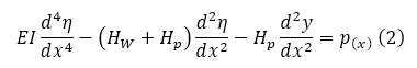
In eq(2), p(x) is the applied load, which can vary within a span. Again we can see that the girder deflection η(x) is a function of cable tension Hw and Hp. It means we need separate calculations for Hw (dead load) to perform live load analysis. Also, Hp is dependent on girder deflection η(x), and we cannot solve eq(2) directly, and we need some kind of iteration.

Melan never provided the solution, and we had to wait until the 20^th century before another genius engineer from Latvia, Leon Moisseiff solved eq(2) (Moisseiff, L., “The Towers, Cables and Stiffening Trusses of the Bridge over the Delaware River between Philadelphia and Camden,” Journal of the Franklin Institute, 1925).