
Author: Seungwoo Lee, Ph.D., P.E., S.E.
Publish Date: 28 Dec, 2021
Dr. Seungwoo Lee has talked about some fundamental differences between linear and nonlinear analysis in structural engineering in the past. In linear analysis, the relationship between the stress and strain of a model is held constant, and the stiffness matrix of the model stays the same throughout the analysis. For a nonlinear analysis, there can be various factors that contribute to its nonlinearities, for example, material yielding, nonlinearities in the boundary conditions, and various forms of geometric nonlinearities. In this article, Dr. Lee will elaborate more on geometric nonlinearities and show how different approaches to approximate geometric nonlinearities can vary the structural analysis results.
- Why do we need to worry about geometric nonlinearities in bridge design?
Say we are to find the top displacement and base moment for the column shown in figure 1. This is a typical case in the column design, with force P resulting from the vertical superstructure reaction and force V resulting from braking force at the fixed bearing location. Calculate the base moment with P = 9726 kips, V = 112.5 kips, L = 148.708 ft. The column is d = 10' -6" reinforced concrete circular section with f'c = 4.5 ksi. (from manual for refined analysis in bridge design and evaluation, FHA)
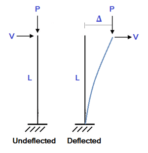
Figure 1. Cantilever column, undeflected and deflected shape. (from What is p-delta analysis? SkyCiv)
In a standard linear static analysis, the base moment and the top deflection can be simply calculated as:
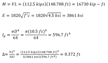
Figure 2 shows the result output from midas Civil linear analysis. You can find the analysis model file here. (EX6_Linear)
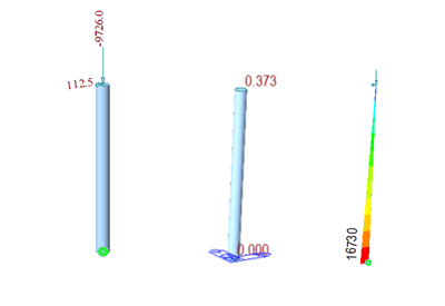 Figure 2. (Left) Loading and boundary conditions. (Middle) Deflection in ft. (Right) Moment in kip-ft.
| Top Deflection (ft) | Base Moment (kip-ft) | |
| Hand Calculation | 0.372 | 16730 |
| EX6_Linear | 0.372 | 16730 |
The results from linear analysis match very well, as shown in table 1. Again, why do we need to worry about nonlinearities? In fact, if P and/or Δ is large, they would be contributing to the generation of secondary moment (M=PΔ) at the base, and we may need more complex analysis.
- Nonlinear analysis assuming "large" displacement
In a simplified P-delta nonlinear analysis,
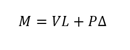 The term PΔ represents the secondary moment induced by the top displacement, and hence given the name "P-delta". This means that the axial force can create additional base moment when we consider the traditional beam bending problem. To calculate the top horizontal deflection Δ, it consists of Δ1 (top horizontal deflection due to horizontal load V) and Δ2 (top horizontal deflection due to vertical load P). To assume Δ = Δ1 + Δ2 is incorrect because the rule of superposition is not valid due to nonlinearities. However, we can calculate Δ and subsequently M as shown below,
Compared to the moment (16730 kip-ft) considering only the linear effect, the base moment obtained considering the secondary effect from the top-displacement is 30.5% higher. Therefore, non-linearity cannot be ignored in this case.
Also, linear analysis assumes that the deflection curve due to P and V is cubic (3rd order). This is only true when P is zero, meaning no axial force is present in an element, and when moment varies linearly within the element. When considering geometric nonlinearity due to axial force, the deflection curves with axial compression and axial tension are not identical.
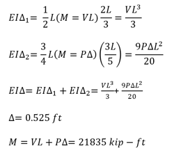
Figure 3 shows the result output from midas Civil nonlinear analysis with the beam modeled with 1 beam element. Figure 4 shows the same analysis but with beam modeled with 10 beam elements. To compile nonlinear analysis in midas Civil, simply go to Analysis -> Analysis Control -> Nonlinear. You can find the analysis model files here. (EX6_Large Displacement and EX6_Large Displacement 10 Division)
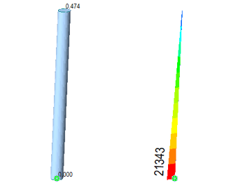 Figure 3. (Left) Deflection in ft. (Right) Moment in kip-ft for the non-linear analysis of the beam modeled with single element.
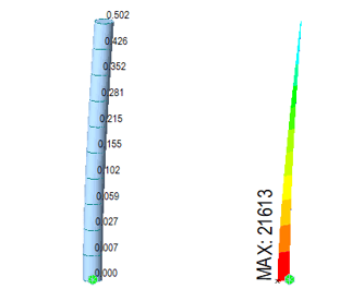
Figure 4. (Left) Deflection in ft (Right) Moment in kip-ft for the non-linear analysis of the beam modeled with 10 beam elements.
Why is the results from 2 midas models different from hand calculation? And why are the analysis results depending on the number of elements? As mentioned above, the deflection curve under axial loads is not cubical. However, most commercial programs, including midas Civil, assume cubical deflection curve for beam elements. This gives good approximation only if no axial force is present in the element or if moment varies linearly between nodes. Therefore, in beam elements the analysis results are independent to the number of divisions if the stiffness is constant, no axial force, and no loads within the element.
However, as shown in the hand calculation above, our cantilever beam has axial force P and the deflection curve is not cubical. Therefore, one cubical curve cannot represent the more complex real deflection curve, and how well the software approximates the real deflection is dependent to the number of divisions. Obviously in the case, 10 elements gives gives better approximation than 1.
- P-Delta Analysis in midas Civil
You can set up analysis control in midas Civil as "P-delta" analysis. However, what is P-delta analysis? How is this option different from the "nonlinear" option that can be found within the same analysis control panel in midas Civil?
One of the confusing parts in nonlinear analysis is the terminology. P-delta analysis is a part of nonlinear analysis, however, it can be interpreted differently depending on engineers. The author prefers to interpret P-delta analysis as finite displacement analysis, as opposed to the "large" displacement analysis discussed previously. According to the midas Civil analysis reference, P-Delta analysis feature in midas Civil produces very accurate
results when lateral displacements are relatively small (within the elastic limit).
In midas Civil, P-delta analysis constitutes equilibrium equations for initial shape but considers the change of axial force and stiffness matrix in each iteration. Therefore, the rule of superposition is not valid again due to the iterative nature.
Figure 5 shows the result output from midas Civil P-delta analysis. To compile P-delta analysis in midas Civil, simply go to Analysis -> Analysis Control -> P-delta. You can find the analysis model file here. (EX6_P-delta)
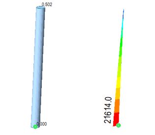
Figure 5. (Left) Deflection in ft. (Right) Moment in kip-ft for the P-delta analysis of the beam.
- Linearized Finite Displacement Analysis
One more method to be mentioned is called linearized finite displacement analysis. In this method, the axial force in each element remains constant, meaning that no iteration is needed. In other words, the rule of superposition is valid and our life is much easier. This method can be applied if the change of the axial force can be ignored and could work for most structures.
Figure 6 shows the result output from midas Civil linearized finite displacement analysis. To define the analysis, you can go to Load -> Initial Forces -> Small Displacement -> Initial Element Forces to add initial forces. You can find the analysis model file here. (EX6 Linearized P-delta)
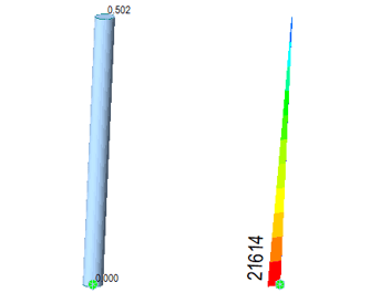 Figure 6. (Left) Deflection in ft. (Right) Moment in kip-ft for the linearized finite displacement analysis of the beam.
We can check this result with hand calculation. Actually, linearized finite displacement method is just considering stiffness reduction (with axial compression) and stiffness increase (with axial tension). The stiffness in the example can be estimated as
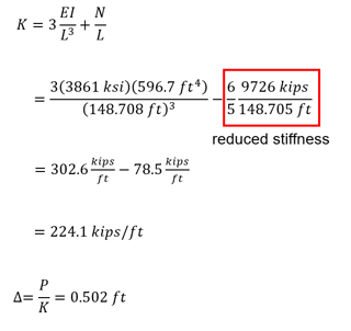
This example is very typical for medium seized bridges. In this case, the stiffness reduction due to axial force is 26% even for a loaded cantilever beam. Therefore, this effect must be considered in the design.
Table 2 below summarizes the result output using different nonlinear analysis options mentioned above. Using single beam element and assuming large displacement for nonlinear analysis (EX6_Large Displacement 1 Element) produces a result that underestimates the load effect. The three other analysis set-ups agree closely with the hand calculations.
| Top Deflection (ft) | Base Moment (kip-ft) | |
|
Hand calculation (simplified P-delta) |
0.525 | 21835 |
|
EX6_Large Displacement (1 element) |
0.474 | 21343 |
| EX6_Large Displacement (10 elements) | 0.502 | 21613 |
| EX6_P-delta | 0.502 | 21614 |
| EX6_Linearized P-delta | 0.502 | 21614 |
|
Hand calculation (Stiffness Reduction) |
0.502 | 21614 |
- Conclusions
What are the findings up to this point? First of all, if there is axial force within the elements, the effects of axial force must be checked even in the medium sized columns. Secondly, there are three levels of analysis methods in geometric nonlinear analysis: large displacement, finite displacement, and linearized finite displacement. In the large and finite displacement, the rule of superposition is not valid, meanwhile linearized finite displacement analysis gives satisfactory results in many cases. Lastly, in nonlinear analysis, even the terminologies can be somewhat confusing and we must clearly understand what the differences are.
Editor: JC Sun
jsun@midasoft.com

Add a Comment